How to evaluate your portfolio performance in 4 steps

By Jakub Svehla

Table of content

Calculating your true return
Measuring the risk
Adjusting the return for the risk
Comparing it to a benchmark

The goal of investing is to maximize your returns while minimizing the risk. So given a level of risk you are willing to accept (your risk profile), you want to maximize the return for that risk. And based on your desired expected risk and return, you need to choose an investing strategy accordingly.

The goal of portfolio performance evaluation is to find out whether your current investment strategy is working. That is, whether your return is appropriate to the risk of your portfolio compared to some common benchmarks.

Thanks to that, it allows you to make better investment decisions. Let’s say that your active investment strategy gives you the same return as the market return (e.g. S&P 500) but with higher risk or higher fees. Then, it would be better to just passively invest in the market instead. On the other hand, if you find out that your portfolio is consistently having higher returns with the same amount of risk as the market (benchmark) with your target risk profile, then you should probably keep your strategy.

There are several metrics to give you the overall picture of the portfolio performance and how it compares to others. So let’s go through them.

Absolute return

Simple return

Absolute total return is your return rate during a given investment period. It tells you how much your investment earned relative to the amount that you invested (cost basis) during your investment period.

The return is calculated as the profit/loss divided by the initial investment (cost basis):

\[ \frac{\text{portfolio value} - \text{amount invested}}{\text{amount invested}} = \frac{\text{profit/loss}}{\text{amount invested}} \]

This formula is called simple return.

Example

Let’s say you invested $100 at the beginning of 2019. At the end of 2021 (after three years), the value of the investment is $130. Then, your return rate is $\frac{130 - 100}{100} = 30\%$.

Annualized return

Using the above formula, you get the return for the whole period you held the investment (holding period return). However, to be able to easily compare your returns to returns of other investments it is usually annualized to give you your average return rate per year (per annum, p.a.). You can annualize your holding period return as follows:

\[ (\text{holding period return} + 1)^{\frac{1}{\text{number of years}}} - 1 \]

Note that we are using a geometric mean to calculate compound annual growth rate (CAGR), which takes into account the effect of compounding, instead of using an arithmetic mean. If we just divided the total return by the number of years (arithmetic mean) we would get an average annual growth rate (AAGR) which overestimates the actual return because it does not take into account the effect of compounding.

Example

Let’s say your total return after three years was 30%. Your average annual return is $(1 + 0.3)^{\frac{1}{3}} - 1 = 9.1\%$ per year. Note that simply dividing the return by 3 would be wrong because investments compound (multiply) so with 10% annual return, you would end up with $\$100 \times 1.1 \times 1.1 \times 1.1 = \$133$ instead of $130. So using the arithmetic mean would overestimate the actual returns.

So far, we have only considered the case where you invest once and don’t do any additional contributions or withdrawals during the holding period. However, when we start adding or removing funds from the portfolio, we cannot use the simple return formula because it would skew the return because each contribution earned money for a different time period. And simple return calculation does not take this into account. So if you added more funds to your portfolio towards the end of the holding period it would falsely underestimate your true return and on the other hand, if you withdrew some funds from the portfolio towards the end of the period it would falsely increase your return.

Example

Let’s say that at the beginning of the year, you buy one share of stock A for $100. At the end of the year, the value of the stock grows to $110. You expect it to grow even more, so you buy 100 more shares for $100 \times \$110 = \$11000$. So your total portfolio value is $11110. That year, the stock grew by 10% again so the ending value of the portfolio was $\$11110 \times 1.1 = \$12221$.

Now, if we calculated the annualized return rate using the simple return rate formula, we would get that our average annual return is $\left(\frac{12221 - 11100}{11100}\right)^{\frac{1}{2}} = 4.9\%$ per year. However, the stock grew by 10% in both years so the average annual return should be 10%.

The reason for the difference is that the simple return assumes that all contributions happened at the beginning of the holding period. But in this case, the second contribution was earning interest only for half of the time but simple return treated it as if it was earning interest both years. So it decreases the actual average return.

Time-weighted return

The solution to this problem is weighing each contribution by the time it was invested and earning money.

We can achieve that by dividing the whole investment period to separate sub-periods starting after each contribution/withdrawals, calculating simple return for each separately, and then linking/chaining/multiplying (compounding) the returns together. This method is called time-weighted return (TWR).

Example

Let’s consider the previous example, where we bought 1 share at $100 the first year and then bought another 100 shares at $110 the next year. So we have two sub-periods. One at the beginning of the first year and second at the beginning of the second year.

The first year, we invested $100 and the value of the investment at the end of the year was $110. So our return rate was $\frac{\$110 - \$100}{\$100} = 10\%$.

At the beginning of the second year, the value of the portfolio was $110 and we invested another $11000 so the total value was $11110. And the value at the end of the second year was $12221. So our return rate for the second year was $\frac{\$12221-\$11110}{\$11110} = 10\%$.

Now we just need to link the sub-period returns together: $(1 + 0.1) \times (1 + 0.1) - 1 = 21\%$.

Now let’s annualize it: $(1 + 0.21)^{\frac{1}{2}} - 1 = 10\%$. Now we get the expected result.

However, there’s one flaw with TWR: It does not take into account the amount of money that was invested at each sub-period. So if you invest more money during the good periods, it will underestimate your return and if you invest more during the bad years, it will underestimate your returns.

Example

Let’s say that we buy 1 share at $100 at the beginning of a year. At the end of the year, the value of the share is $130. So our return is 30% per year. Since we believe it will grow at the same rate next year, we will buy another 100 shares at $130. So now, the value of the portfolio is $\$130 + (100 \times \$130) = \$13130$.

However, the next year the value of the stock goes down by 10% and the value of the portfolio at the end of the year is $11817. So we are at loss of $1313.

If we calculate our TWR, we get $1.3 \times 0.9 = 17\%$. So we get a high positive return even though we are at loss of $1313.

Money-weighted return

As we have seen in the previous example, TWR does not take the amounts and timing of cashflows into account. However, cashflow timing matters and can have big impact on your return.

To calculate your actual return, considering your actual cashflows, money-weighted return (MWR) is used.

One way to calculate the MWR is by using internal rate or return calculation (IRR). The Internal Rate of Return (IRR) is the discount rate that makes the net present value (NPV) of all portfolio’s cashflows zero:

\[ \text{NPV} = \sum^N_{n=0}\frac{C_n}{(1 + r)^n} = 0 \]

$N$ is the number of time periods and $C_n$ is the cashflow at the beginning of the period $n = 0 \dots N$.

However, I find this formula confusing. I think using the equivalent compounding formula (net future value) instead of the discounting formula makes it easier to understand what it calculates:

\[ \text{NFV} = \sum^N_{n=0} C_n \left(1 + r\right)^{N-n} = 0 \]

Now we need to solve the equation to get the $r$ which is our return rate. Unfortunately, there is no analytical formula to calculate it, so we need to calculate it numerically (iteratively by trial and error). For this reason, it’s difficult to calculate by hand. However, in Excel or Google Sheets, we can use XIRR function to calculate it.

Example

Let’s consider the previous example, where we invested $100 the first year, then $13000 the second year, and the value of the portfolio at the beginning of the third year was $11817. So we have the following cash flows:

If we plug the cashflows into the formula, we get:

\[ -100 (1 + r)^2-13000(1+r)^1+11817(1+r)^0=0 \]

That equals to:

\[ 11817 = 100(1+r)^2+13000(1+r) \]

So the ending portfolio balance is equal to the first cash flow earning compounding interest for two years plus the second cash flow earning interest for one year.

To solve the equation, we can plug the cashflows into Google Sheets or Excel and use the IRR function:

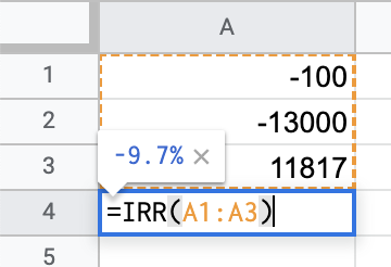
And we see that our actual return was -9.7% which is kind of expected because the second year with -10% return had the largest weight while the first year with +30% return had a little weight and so it increased the average only by little.

TWR vs MWR

TODO

Risk measures

TODO

Risk adjusted return

TODO

Relative return

TODO

Conclusion

TODO

If you found the post useful I would be super happy if you shared it with others!